Getting starting with the varPro R-package for model-independent variable selection in regression, classification, survival and unsupervised settings
Min Lu (luminwin@gmail.com)
Aster Shear (aster.shear@gmail.com)
Udaya B. Kogalur (ubk@kogalur.com)
Hemant Ishwaran
(hemant.ishwaran@gmail.com)
2025-04-22
getstarted.Rmd
Overview
VarPro is a novel method for variable selection based on rule-based
models. These include decision rules, decision trees, Bayesian Adaptive
Regression Trees (BART), Bayesian forests, and random forests. Such
rule-based procedures do not require predefined model specifications and
can accommodate a variety of outcome types, including regression,
classification, survival, and longitudinal data. The current
implementation of the VarPro software uses rules extracted from random
forests via the randomForestSRC package.
Traditional variable selection methods, such as permutation variable importance (VIMP) [1–3] and knockoffs [4], have known limitations. Both rely on generating artificial covariates, which can lead to unreliable results when these synthetic variables fail to reflect the structure of the original data.
VarPro takes a different approach. Rather than introducing artificial covariates, it constructs release rules that selectively relax variable constraints to evaluate how each variable influences the response. By working within local neighborhoods defined by observed data, VarPro avoids the pitfalls of synthetic variable generation and provides a robust, flexible framework for assessing variable importance. Like VIMP and knockoffs, it makes no assumptions about the conditional distribution of the response.
How VarPro Works
The VarPro algorithm proceeds in two main stages:
- Guided Tree Splitting
A forest of
ntreetrees is grown using guided splitting, where variables are selected with probability based on their split-weights.This process encourages rules that are more likely to involve influential variables.
- Rule Harvesting
A random subset of
max.treetrees is selected.From each of these trees, a subset of
max.rules.treebranches (rules) is sampled.
- VarPro Importance
The importance of a variable is calculated by comparing local estimators of a target function within a rule-defined region and a released version of that region (for example, in regression, , so , and in classification, for class , so ).
For each rule, VarPro computes the sample average of the outcome in the region defined by the rule, and compares it to the average in a released region—one where constraints on the variable(s) being tested are removed.
-
The importance score for a variable (or set of variables) is the absolute difference between these two local averages:
where:
- is the average of in the original region,
- is the average in the released region with variable(s) in unconstrained.
This process is repeated across multiple rules, and the final VarPro importance is a weighted average.
Because VarPro uses only observed data—no artificial permutations or synthetic features—it avoids biases that affect other variable importance methods such as permutation importance and knockoffs.
The current version of the software applies a modification where the Importance is locally standardized. This is now used for the default setting.
VarPro is applicable to:
Regression
Multivariate regression
Multiclass classification
Survival analysis
A new mode now handles unsupervised data
Split-Weights
Guided splitting depends on split-weights, which determine how often a variable is chosen for splitting. By default, these weights are derived using a combination of lasso regression, shallow trees, and in some instances, permutation importance.
The split-weight of a variable is defined as the absolute standardized lasso coefficient, multiplied by its frequency in a forest of shallow trees.
If the sample size and number of features are moderate, split-weights may instead rely on permutation importance.
To use lasso effectively, all variables (including factors) are converted to real-valued features via one-hot encoding.
You can customize how
split-weights are computed using the
split.weight.method option:
“lasso” – Use only lasso coefficients.
“lasso tree” – Combine lasso with tree-based importance.
“lasso vimp” – Combine lasso with permutation importance.
Variable Selection and Thresholding
Variables are ranked based on their VarPro importance scores. Larger values indicate more influential features. You can use cross-validation) to select a threshold for identifying relevant variables.
Performance and Customization
For faster runtimes, use fewer trees (
ntree) and increase the minimum terminal node size (nodesize).Additional tuning options are available. See the examples section for more details.
Handling Class Imbalance
For binary classification tasks with class imbalance, VarPro
automatically uses Random Forest Quantile Classification (RFQ) [5, 6]. This behavior can be overridden with the
use.rfq option.
Quick Start
Quick Installation
Like many other R packages, the simplest way to obtain
randomForestSRC is to install it directly from CRAN or
Github via typing the following command in R console:
# install.packages("devtools")
devtools::install_github("kogalur/varPro")

# another way
install.packages("varPro", repos = "https://cran.us.r-project.org")
A Quick Example of Regression
library(varPro)

## check the data
data(Boston, package = "MASS")
head(Boston)

>      crim zn indus chas   nox    rm  age    dis rad tax ptratio  black lstat medv
> 1 0.00632 18  2.31    0 0.538 6.575 65.2 4.0900   1 296    15.3 396.90  4.98 24.0
> 2 0.02731  0  7.07    0 0.469 6.421 78.9 4.9671   2 242    17.8 396.90  9.14 21.6
> 3 0.02729  0  7.07    0 0.469 7.185 61.1 4.9671   2 242    17.8 392.83  4.03 34.7
> 4 0.03237  0  2.18    0 0.458 6.998 45.8 6.0622   3 222    18.7 394.63  2.94 33.4
> 5 0.06905  0  2.18    0 0.458 7.147 54.2 6.0622   3 222    18.7 396.90  5.33 36.2
> 6 0.02985  0  2.18    0 0.458 6.430 58.7 6.0622   3 222    18.7 394.12  5.21 28.7

## call varpro
o <- varpro(medv ~ ., data = Boston)

## extract and print importance values
imp <- importance(o)
print(imp)

>                 z
> rm      2.8020301
> lstat   2.4851461
> nox     1.7625229
> ptratio 1.6138725
> dis     1.2464620
> crim    1.1134819
> b       0.8257784
> tax     0.1076922
> indus   0.0581391
> age     0.0000000
> chas    0.0000000
> rad     0.0000000

## plot importance values
importance(o, plot.it = TRUE)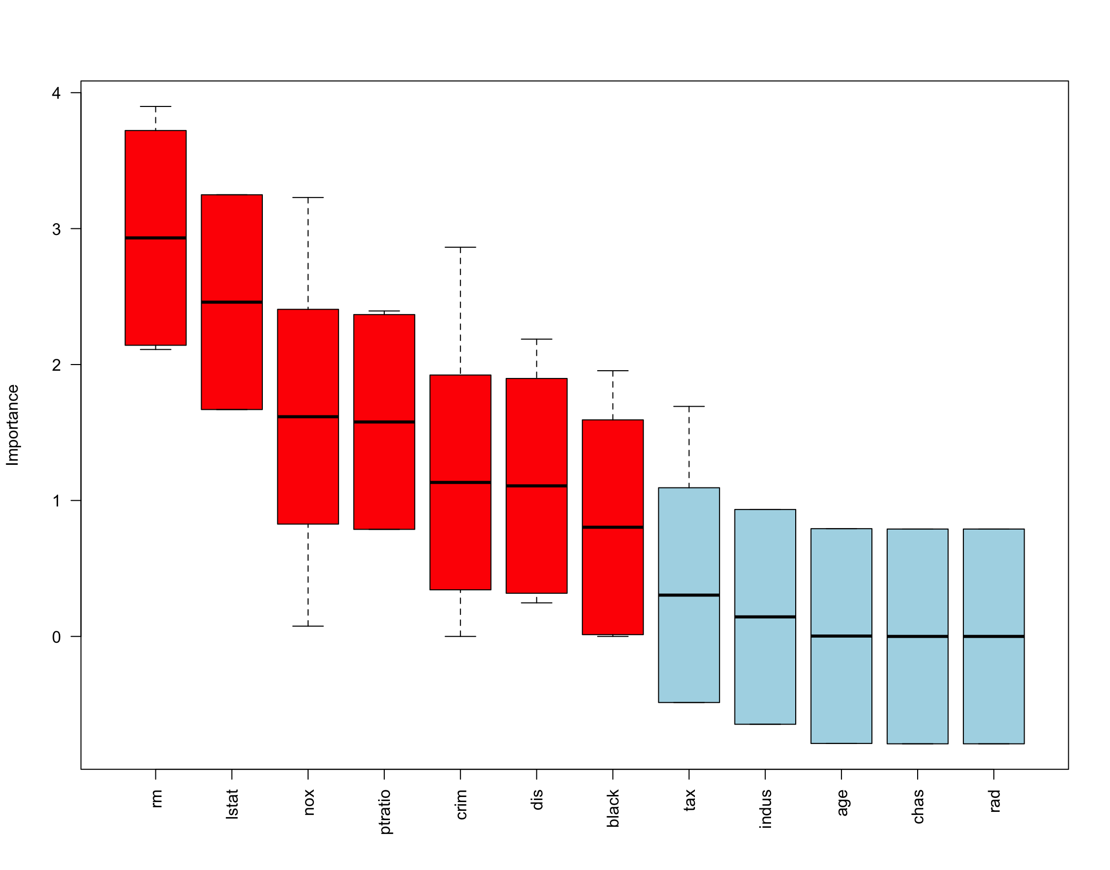
In the
above output, print(imp) display the VarPro importance.
In the above figure, important variables are marked in red color while noise variables are marked in blue color.
Note that not all of the variables will be listed nor plotted in the output since the varPro algorithm prefilters noise variables before calculating the importance values.
Cross-validated Cutoff Value for VarPro
To tune the cutoff value of VarPro for the final variable selection decision, our package also provides a function to fit a random forest model in a forward fitting fashion where variables were added in to the model according to a grid of cutoff values. The optimal subset of variables is defined by the random forest model with the smallest out-of-bag error.
o <- cv.varpro(medv ~ ., data = Boston)
print(o)

$imp
  variable         z
1    lstat 3.6781189
2       rm 3.4421867
3  ptratio 2.0686261
4      nox 1.2541217
5     crim 1.2162352
6      dis 1.0108895
7    black 0.4816799

$imp.conserve
  variable        z
1    lstat 3.678119
2       rm 3.442187
3  ptratio 2.068626
4      nox 1.254122

$imp.liberal
  variable         z
1    lstat 3.6781189
2       rm 3.4421867
3  ptratio 2.0686261
4      nox 1.2541217
5     crim 1.2162352
6      dis 1.0108895
7    black 0.4816799

$err
          zcut nvar       err          sd
[1,] 0.1000000    7 0.2039396 0.008710617
[2,] 0.4877551    6 0.2162618 0.011050992
[3,] 1.0306122    5 0.2155826 0.009447152
[4,] 1.2244898    4 0.2052468 0.013659195
[5,] 1.2632653    3 0.2399562 0.014592443

$zcut
[1] 0.1

$zcut.conserve
[1] 1.22449

$zcut.liberal
[1] 0.1
In the above output, lines for $imp display the final
list of variables that minimize out-of-sample error rate of a random
forest, where the error rates were listed in lines for
$error. Its cutoff value for the VarPro standardized
importance is listed in lines for $zcut. Lines for
$imp.conserve and $imp.liberal display a
“conservative” and “liberal” list of variables returned using a one
standard deviation rule. The conservative list comprises variables using
the largest cutoff with error rate within one standard deviation from
the optimal cutoff error rate, whereas the liberal list uses the
smallest cutoff value with error rate within one standard deviation of
the optimal cutoff error rate.
More examples for regression, classification, survival and unsupervised problems
Regression with hot-encoding
## load the data
data(BostonHousing, package = "mlbench")
head(BostonHousing)

     crim zn indus chas   nox    rm  age    dis rad tax ptratio      b lstat medv
1 0.00632 18  2.31    0 0.538 6.575 65.2 4.0900   1 296    15.3 396.90  4.98 24.0
2 0.02731  0  7.07    0 0.469 6.421 78.9 4.9671   2 242    17.8 396.90  9.14 21.6
3 0.02729  0  7.07    0 0.469 7.185 61.1 4.9671   2 242    17.8 392.83  4.03 34.7
4 0.03237  0  2.18    0 0.458 6.998 45.8 6.0622   3 222    18.7 394.63  2.94 33.4
5 0.06905  0  2.18    0 0.458 7.147 54.2 6.0622   3 222    18.7 396.90  5.33 36.2
6 0.02985  0  2.18    0 0.458 6.430 58.7 6.0622   3 222    18.7 394.12  5.21 28.7

## convert some of the features to factors
Boston <- BostonHousing
Boston$zn <- factor(Boston$zn)
Boston$chas <- factor(Boston$chas)
Boston$lstat <- factor(round(0.2 * Boston$lstat))
Boston$nox <- factor(round(20 * Boston$nox))
Boston$rm <- factor(round(Boston$rm))

## call varpro and print the importance
print(importance(o <- varpro(medv~., Boston)))
                 z
rm8     5.47876912
lstat1  2.84240815
rm6     2.62702059
lstat2  1.96640588
rm7     1.93009100
crim    1.91978125
nox14   1.90744534
ptratio 1.48896289
tax     1.04818974
nox13   0.99046707
b       0.73989233
indus   0.68380574
lstat5  0.66820269
dis     0.59586207
age     0.44459518
nox10   0.28498938
lstat0  0.27933331
lstat4  0.24870583
lstat6  0.04865196
chas    0.01651904
nox11   0.00000000
nox12   0.00000000
nox17   0.00000000
rad     0.00000000
rm9     0.00000000
zn90    0.00000000

## get top variables
get.topvars(o)
 [1] "rm8"     "rm6"     "lstat1"  "nox14"   "crim"    "lstat2"  "rm7"     "ptratio" "nox13"
[10] "tax"     "dis"     "b"       "indus"   "age"     "lstat5"  "lstat0"  "nox10"   "lstat4"
[19] "lstat6"  "chas"    "nox11"   "nox12"   "nox17"   "rad"     "rm9"     "zn90"

## map importance values back to original features
print(get.orgvimp(o))
   variable         z
6        rm 5.6336672
13    lstat 2.7783778
5       nox 2.0679178
1      crim 1.9483674
11  ptratio 1.5227539
10      tax 1.0942222
12        b 0.7622109
8       dis 0.6932214
3     indus 0.6729344
7       age 0.4207372
2        zn 0.0000000
4      chas 0.0000000
9       rad 0.0000000

## same as above ... but for all variables
print(get.orgvimp(o, pretty = FALSE))
     crim        zn     indus      chas       nox        rm       age       dis       rad       tax
1.8527969 0.0000000 0.6973291 0.0000000 1.7652739 5.6260698 0.5494061 1.0707970 0.0000000 1.1394922
  ptratio         b     lstat
1.4486139 0.9302271 2.7298017
Multivariate regression
data(BostonHousing, package = "mlbench")

## using cbind multivariate formula call
importance(varpro(cbind(lstat, nox) ~., BostonHousing))
[[1]]
                z
medv    2.8373757
rm      2.2395107
indus   1.4832981
age     1.4434773
dis     1.1467323
crim    0.8905107
tax     0.2178625
b       0.0000000
ptratio 0.0000000
rad     0.0000000
zn      0.0000000

[[2]]
                z
indus   3.6984597
dis     3.1230747
crim    2.1167525
age     1.7821251
medv    1.3248673
rm      1.0124103
tax     0.7094792
b       0.0000000
ptratio 0.0000000
rad     0.0000000
zn      0.0000000

## equivalent as using rfsrc multivariate formula call
# importance(varpro(Multivar(lstat, nox) ~., BostonHousing))
Classification
# use the iris data as an example. Check the data:
head(iris)
  Sepal.Length Sepal.Width Petal.Length Petal.Width Species
1          5.1         3.5          1.4         0.2  setosa
2          4.9         3.0          1.4         0.2  setosa
3          4.7         3.2          1.3         0.2  setosa
4          4.6         3.1          1.5         0.2  setosa
5          5.0         3.6          1.4         0.2  setosa
6          5.4         3.9          1.7         0.4  setosa
## apply varpro to the iris data
o <- varpro(Species ~ ., iris)

## call the importance function and print the results
print(importance(o))

$unconditional
                    z
Petal.Length 3.292862
Petal.Width  3.252240
Sepal.Width  0.000000

$conditional.z
                setosa versicolor virginica
Petal.Length 0.2048927   5.536114  1.794192
Petal.Width  4.9433575   6.056593  3.723534
Sepal.Width  0.0000000   0.000000  0.000000
Survival
data(pbc, package = "randomForestSRC")
head(pbc)

  days status treatment   age sex ascites hepatom spiders edema bili chol albumin copper    alk   sgot
1  400      1         1 21464   1       1       1       1   1.0 14.5  261    2.60    156 1718.0 137.95
2 4500      0         1 20617   1       0       1       1   0.0  1.1  302    4.14     54 7394.8 113.52
3 1012      1         1 25594   0       0       0       0   0.5  1.4  176    3.48    210  516.0  96.10
4 1925      1         1 19994   1       0       1       1   0.5  1.8  244    2.54     64 6121.8  60.63
5 1504      0         2 13918   1       0       1       1   0.0  3.4  279    3.53    143  671.0 113.15
6 2503      1         2 24201   1       0       1       0   0.0  0.8  248    3.98     50  944.0  93.00
  trig platelet prothrombin stage
1  172      190        12.2     4
2   88      221        10.6     3
3   55      151        12.0     4
4   92      183        10.3     4
5   72      136        10.9     3
6   63       NA        11.0     3


o <- varpro(Surv(days, status)~., pbc)
print(importance(o))

                    z
bili        2.4223890
edema       1.6002777
copper      1.2203896
ascites     1.0023466
albumin     0.9590398
prothrombin 0.8745652
age         0.6094406
stage       0.3043256
chol        0.0000000
hepatom     0.0000000
sgot        0.0000000
See more survival problems.
Unsupervised clustering
data(BostonHousing, package = "mlbench")

## default call
o <- uvarpro(BostonHousing)
print(importance(o))

             mean       std         z
indus   0.5889298 0.3465154 1.6995778
nox     0.5324178 0.3993524 1.3332031
medv    0.4519824 0.4315267 1.0474030
tax     0.3339766 0.3590255 0.9302308
rad     0.3264583 0.3538616 0.9225594
zn      0.3686787 0.4057892 0.9085474
crim    0.3380561 0.4019666 0.8410055
lstat   0.3248712 0.4206612 0.7722872
dis     0.2526544 0.3832465 0.6592476
ptratio 0.1881419 0.3276218 0.5742654
age     0.1946974 0.3572511 0.5449876
rm      0.1481955 0.3230311 0.4587656
b       0.0000000 0.0000000       NaN
chas    0.0000000 0.0000000       NaN
See more unsupervised problems.
Different split-weight methods
We can use different split-weight methods:
## ----------------------------------------------------------------------
## high dimensional survival example using different split-weight methods
## ----------------------------------------------------------------------
data(vdv, package = "randomForestSRC")
vdv[1:5,1:17]
   Time Censoring AA555029_RC AA598803_RC     AB002301   AB002308   AB002331  AB002351    AB002445
1 12.53         0  -0.5049331  -0.2425008 -0.199315682 0.90024251  0.6311663 -0.601269  0.44181645
2  6.44         0  -0.5879813   0.4384945 -0.621200562 0.09301399  0.9500715 -1.484902  0.21924725
3 10.66         0  -0.3521244  -0.2258911  0.006643856 0.13952097 -0.7275022 -1.043085 -0.27572003
4 13.00         0  -0.4750357   0.5016111 -0.671029449 0.76404345 -0.9234960 -1.926718 -0.01993157
5 11.98         0  -0.1660964   0.1361991  0.989934564 0.62452251  0.9168522 -1.455004  0.07972627
     AB002448    AB004064   AB004857   AB006625    AB006628    AB006746    AB007458    AB007855
1 -0.26575425 -2.80370736  0.1328771 -1.1427432 -0.52818656 -0.97000301  0.32222703  0.41856295
2  0.14616483  0.08637013  0.5913032  1.1859283 -0.70424873 -0.62120056  0.33883667  0.05979471
3 -0.49496728  0.56140584  0.7108926  1.2424011 -0.77068734  1.12613368 -0.38534367 -0.23253496
4  0.09301399  0.41524100  0.2425008 -0.9002425  0.07972627 -0.43517259  0.05315085 -1.56795001
5  0.77733117  0.19267184 -0.3720559 -0.9700030 -0.41856295 -0.07640435 -0.20263761  0.54147428


f <- as.formula(Surv(Time, Censoring)~.)

## lasso only
print(importance(varpro(f, vdv, split.weight.method = "lasso")))

                       z
Contig28552_RC 1.4208629
NM_020974      1.0405454
Contig47405_RC 0.6928171


## lasso and vimp
print(importance(varpro(f, vdv, split.weight.method = "lasso vimp")))

                       z
NM_020974      0.9678159
Contig28552_RC 0.9466678
U45975         0.6766980
Contig43983_RC 0.5508783
Contig47405_RC 0.4033919
NM_014181      0.2864786
AB020689       0.0000000

## lasso, vimp and shallow trees
print(importance(varpro(f, vdv, split.weight.method = "lasso vimp tree")))

                       z
NM_020974      1.1038727
Contig28552_RC 0.9501651
Contig43983_RC 0.7836134
Contig47405_RC 0.5493373
AB020689       0.3757536
U45975         0.3738694
Contig25290_RC 0.3589115
Contig55574_RC 0.0000000
NM_003108      0.0000000
NM_006681      0.0000000
NM_014181      0.0000000
Customized split-weights
## load the data
data(BostonHousing, package = "mlbench")

## make some features into factors
Boston <- BostonHousing
Boston$zn <- factor(Boston$zn)
Boston$chas <- factor(Boston$chas)
Boston$lstat <- factor(round(0.2 * Boston$lstat))
Boston$nox <- factor(round(20 * Boston$nox))
Boston$rm <- factor(round(Boston$rm))

## get default custom split-weights: a named real vector
swt <- varPro:::get.splitweight.custom(medv~., Boston)
swt
   crim   indus     age     dis     rad     tax ptratio       b     zn0  zn12.5  zn17.5    zn18
      1       1       1       1       1       1       1       1       1       1       1       1
   zn20    zn21    zn22    zn25    zn28    zn30    zn33    zn34    zn35    zn40    zn45  zn52.5
      1       1       1       1       1       1       1       1       1       1       1       1
   zn55    zn60    zn70    zn75    zn80  zn82.5    zn85    zn90    zn95   zn100    chas    nox8
      1       1       1       1       1       1       1       1       1       1       1       1
   nox9   nox10   nox11   nox12   nox13   nox14   nox15   nox17     rm4     rm5     rm6     rm7
      1       1       1       1       1       1       1       1       1       1       1       1
    rm8     rm9  lstat0  lstat1  lstat2  lstat3  lstat4  lstat5  lstat6  lstat7  lstat8
      1       1       1       1       1       1       1       1       1       1       1

## define custom splits weight
swt <- swt[grepl("crim", names(swt)) |
           grepl("zn", names(swt)) |
           grepl("nox", names(swt)) |
           grepl("rm", names(swt)) |
           grepl("lstat", names(swt))]

swt[grepl("nox", names(swt))] <- 4
swt[grepl("lstat", names(swt))] <- 4

swt <- c(swt, strange=99999)

cat("custom split-weight\n")
print(swt)

   crim   indus     age     dis     rad     tax ptratio       b     zn0  zn12.5  zn17.5    zn18
      1       1       1       1       1       1       1       1       1       1       1       1
   zn20    zn21    zn22    zn25    zn28    zn30    zn33    zn34    zn35    zn40    zn45  zn52.5
      1       1       1       1       1       1       1       1       1       1       1       1
   zn55    zn60    zn70    zn75    zn80  zn82.5    zn85    zn90    zn95   zn100    chas    nox8
      1       1       1       1       1       1       1       1       1       1       1       4
   nox9   nox10   nox11   nox12   nox13   nox14   nox15   nox17     rm4     rm5     rm6     rm7
      4       4       4       4       4       4       4       4       1       1       1       1
    rm8     rm9  lstat0  lstat1  lstat2  lstat3  lstat4  lstat5  lstat6  lstat7  lstat8 strange
      1       1       4       4       4       4       4       4       4       4       4   99999


## call varpro with the custom split-weights
o <- varpro(medv~.,Boston,split.weight.custom=swt,verbose=TRUE,sparse=FALSE)
cat("varpro result\n")
print(importance(o))

                z
lstat1 3.80058227
nox14  2.52599762
lstat2 2.40081592
nox13  2.26405255
lstat3 2.20891414
nox10  1.57659854
lstat5 1.53197178
crim   1.23040167
lstat0 1.21195016
nox11  1.14235212
lstat4 0.95613610
nox12  0.93286170
lstat6 0.76143191
nox9   0.56287351
nox8   0.47674733
zn20   0.45050785
zn0    0.40524283
nox15  0.24961443
nox17  0.20264288
zn25   0.17448268
zn22   0.02993067
lstat7 0.00000000
zn12.5 0.00000000
zn21   0.00000000
zn28   0.00000000
zn30   0.00000000
zn33   0.00000000
Cite this vignette as
M. Lu, A. Shear, U. B.
Kogalur, and H. Ishwaran. 2025. “varPro: getting started with varPro
vignette.” https://www.varprotools.org/articles/getstarted.html.
@misc{LuGettingStartedvarpro,
    author = "Min Lu and Aster Shear and Udaya B. Kogalur and Hemant Ishwaran",
    title = {{varPro}: getting started with {varPro} vignette},
    year = {2025},
    url = {http://www.varprotools.org/articles/getstarted.html},
    howpublished = "\url{http://www.varprotools.org/articles/getstarted.html}",
    note = "[accessed date]"
}