Individual Variable Priority (iVarPro)

Min Lu (luminwin@gmail.com)

Aster Shear (aster.shear@gmail.com)

Udaya B. Kogalur (ubk@kogalur.com)

Hemant Ishwaran (hemant.ishwaran@gmail.com)

2026-03-31

Understanding individual-level variable importance is essential for personalized modeling, yet it remains underexplored in traditional statistical and machine learning methods.

Most approaches assess variable importance at the population level, which can mask the heterogeneity of effects across individuals. In applications where personalized decisions are critical—such as precision medicine, targeted marketing, or individualized risk prediction—this can be a major limitation.

Enter iVarPro: Localized Gradient-Based Importance

iVarPro extends VarPro by defining individual-level feature importance through local gradients.

• The gradient reflects how small changes in a variable affect the predicted outcome for a specific individual.

• This provides a natural and interpretable measure of a variable’s influence on an individual prediction—essentially a personalized sensitivity analysis.

How iVarPro Works

iVarPro builds on the structural consistency of VarPro’s rules [1]:

1. Regions $R$ defined by VarPro rules identify meaningful neighborhoods in the feature space.

2. Within each region, iVarPro fits a local linear regression to estimate the gradient of the outcome with respect to each variable.

3. However, data within a single region is often sparse—leading to unstable estimates.

To solve this, iVarPro uses release regions:

• A release region loosens the constraint on a specific variable $S$ while keeping all others fixed.

• This targeted expansion injects the variation needed along $S$ to accurately compute the directional derivative.

• The result: a more stable, interpretable, and localized measure of individual variable importance.

R example of case-specific importance matrix and visualization

data(peakVO2, package = "randomForestSRC")
o <- varpro(Surv(ttodead, died) ~ .,
            peakVO2, ntree = 50)
ivp <- ivarpro(o)
print(ivp[1:5, 1:8])

##      age    gender bmi   peak.vo2 chemo  
## [1,]  0.041  NA  0.028   0.312   NA    
## [2,]  NA     NA  0.011   0.284   0.022  
## [3,]  0.014  0.031  NA   0.271   NA    
## [4,]  0.033  NA  0.019   0.290   0.017  

ivarpro returns an $N\times p$ matrix of case-specific importance values. NA = variable not important for that case.

imp <- ivarpro(o, cut.max = 2, adaptive = FALSE)
shap.ivarpro(imp)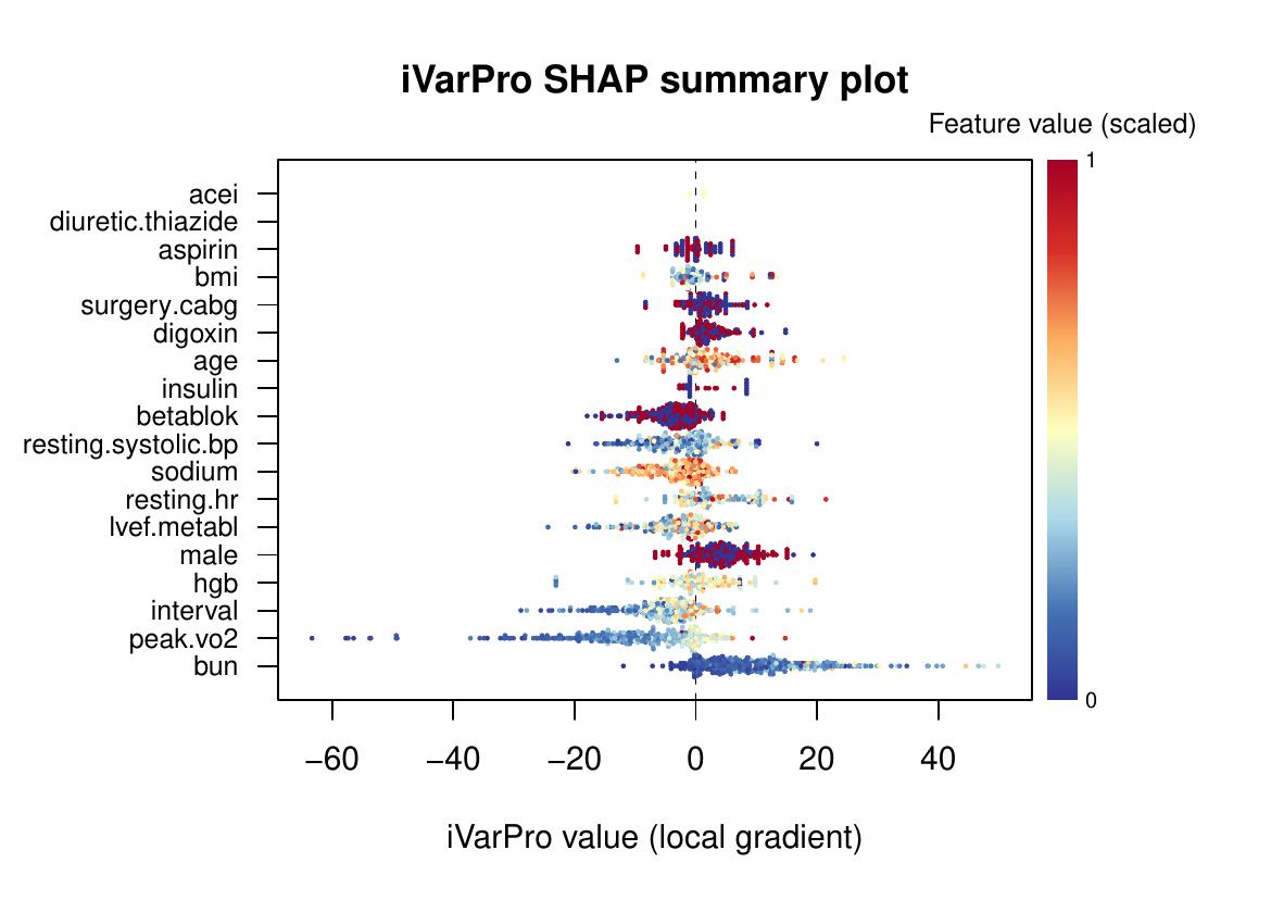

The shap.ivarpro function provides SHAP-like beeswarm plot: each dot = one case, color = feature value, x-axis = individualized importance.

partial.ivarpro(imp, var = "peak.vo2",
                col.var = "interval",
                size.var = "y")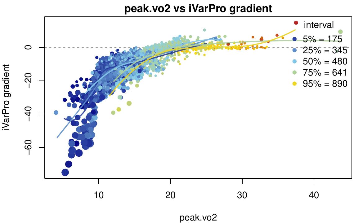

The partial.ivarpro function provides case-specific importance for peak.vo2, points colored by interval, sized by outcome y.

R example of a 2-signal simulation

## true regression function
true.function <- function(which.simulation) {
  if (which.simulation == 1) {
    function(x1,x2) {1*(x2<=.25) +
        15*x2*(x1<=.5 & x2>.25) + (7*x1+7*x2)*(x1>.5 & x2>.25)}
  }
  else if (which.simulation == 2) {
    function(x1,x2) {r=x1^2+x2^2;5*r*(r<=.5)}
  }
  else {
    function(x1,x2) {6*x1*x2}
  }
}

## simulation function
simfunction = function(n = 1000, true.function, d = 20, sd = 1) {
  d <- max(2, d)
  X <- matrix(runif(n * d, 0, 1), ncol = d)
  dta <- data.frame(list(x = X, y = true.function(X[, 1], X[, 2]) + rnorm(n, sd = sd)))
  colnames(dta)[1:d] <- paste("x", 1:d, sep = "")
  dta
}

## iVarPro importance plot
ivarpro.plot <- function(dta, release=1, combined.range=TRUE,
                         cex=1.0, cex.title=1.0, sc=5.0, gscale=30, title=NULL) {
  x1 <- dta[,"x1"]
  x2 <- dta[,"x2"]
  x1n = expression(x^{(1)})
  x2n = expression(x^{(2)})
  if (release==1) {
    if (is.null(title)) title <- bquote("iVarPro Estimated Gradient " ~ x^{(1)})
    cex.pt <- dta[,"Importance.x1"]
  }
  else {
    if (is.null(title)) title <- bquote("iVarPro Estimated Gradient " ~ x^{(2)})
    cex.pt <- dta[,"Importance.x2"]
  }
  if (combined.range) {
    cex.pt <- cex.pt / max(dta[, c("Importance.x1", "Importance.x2")],na.rm=TRUE)
  }
  rng <- range(c(x1,x2))
  par(mar=c(4,5,5,1),mgp=c(2.25,1.0,0))
  par(bg="white")
  gscalev <- gscale
  gscale <- paste0("gray",gscale)
  plot(x1,x2,xlab=x1n,ylab=x2n,
       ylim=rng,xlim=rng,
       col = "#FFA500", pch = 19,
       cex=(sc*cex.pt),cex.axis=cex,cex.lab=cex,
       panel.first = rect(par("usr")[1], par("usr")[3], par("usr")[2], par("usr")[4], 
                          col = gscale, border = NA))
  abline(a=0,b=1,lty=2,col= if (gscalev<50) "white" else "black")
  mtext(title,cex=cex.title,line=.5)
}

## simulate the data
which.simulation <- 1
df <- simfunction(n = 500, true.function(which.simulation))

## varpro analysis
o <- varpro(y~., df)

## canonical ivarpro analysis
imp1 <- ivarpro(o)

## ivarpro analysis with custom lambda
imp2 <- ivarpro(o, cut = seq(.05, .75, length=21))

## build data for plotting the results
df.imp1 <- data.frame(Importance = imp1, df[,c("x1","x2")])
df.imp2 <- data.frame(Importance = imp2, df[,c("x1","x2")])

## plot the results
par(mfrow=c(2,2))
ivarpro.plot(df.imp1,1)
ivarpro.plot(df.imp1,2)
ivarpro.plot(df.imp2,1)
ivarpro.plot(df.imp2,2)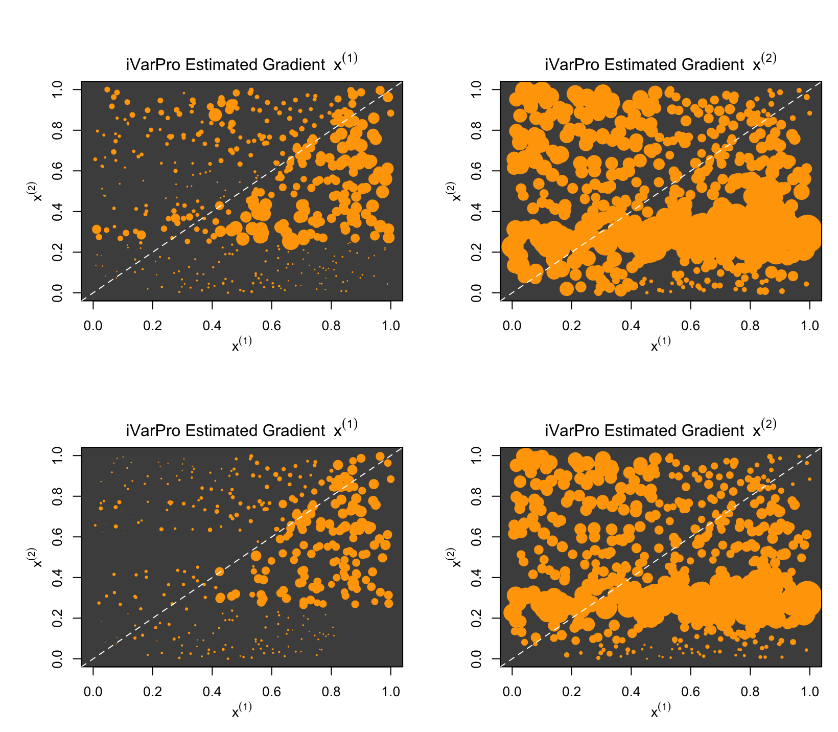

Cite this vignette as
M. Lu, A. Shear, U. B. Kogalur, and H. Ishwaran. 2025. “ivarPro: individual variable priority vignette.” http://www.varprotools.org/articles/ivarpro.html.

@misc{LuVarProi,
    author = "Min Lu and Aster Shear and Udaya B. Kogalur and Hemant Ishwaran",
    title = {{ivarPro}: individual variable priority vignette},
    year = {2025},
    url = {http://www.varprotools.org/articles/ivarpro.html},
    howpublished = "\url{http://www.varprotools.org/articles/ivarpro.html}",
    note = "[accessed date]"
}

1. Lu M, Ishwaran H. Individual variable priority: A model-independent local gradient method for variable importance. Artificial Intelligence Review. 2025;58:407.