isopro to Identify Anomalous Data

Min Lu (luminwin@gmail.com)

Aster Shear (aster.shear@gmail.com)

Udaya B. Kogalur (ubk@kogalur.com)

Hemant Ishwaran (hemant.ishwaran@gmail.com)

2025-04-29

The isopro function implements Isolation Forests (Liu et al., 2008) [1], a random forest-based technique designed for anomaly detection.

Unlike traditional methods, Isolation Forests use randomly constructed trees and leverage the concept of early isolation: rare or anomalous observations tend to split away from the rest of the data quickly under random partitioning.

How It Works

• Trees are built using pure random splitting.

• Each tree is trained on a small subsample of the data—typically much smaller than the 63.2% subsample rate used in traditional random forests.

• The key idea: anomalous observations isolate faster, meaning they appear in terminal nodes at shallower depths.

• The depth of an observation (i.e., number of splits before reaching a terminal node) becomes a natural anomaly score—shallower = more anomalous.

How to Use isopro

There are three main ways to run isopro:

1. Unsupervised Analysis (most common)

• Use the data argument only.

• Set the method option to control how trees are built ("rnd", "unsupv", or "auto").

2. Supervised Analysis (less common)

• Provide both a formula and a data set.

• In this case, the analysis is supervised and the method option is ignored.

3. Using a VarPro Object (advanced)

• Pass a fitted VarPro object directly.

• This applies isolation forests to the dimension-reduced feature space produced by VarPro (e.g., from a previous method = "unsupv" run).

• This is similar to the unsupervised mode but benefits from prior dimensionality reduction.

Choosing a Method

The method option determines how trees are constructed:

• “rnd” (pure random splitting):

  • Fastest method

  • Often effective, but not always optimal

• “unsupv” (unsupervised tree splitting):

  • A balance of speed and structure

  • Works well in many cases

• “auto” (auto-encoder splitting):

  • Most powerful, but slowest

  • Best suited for low-dimensional problems

We recommend experimenting with different methods, especially if your data has unique structure or high-dimensional features. See the simulation example below:

R Examples

## monte carlo parameters
nrep <- 25
n <- 1000

## simulation function
twodimsim <- function(n=1000) {
  cluster1 <- data.frame(
    x = rnorm(n, -1, .4),
    y = rnorm(n, -1, .2)
  )
  cluster2 <- data.frame(
    x = rnorm(n, +1, .2),
    y = rnorm(n, +1, .4)
  )
  outlier <- data.frame(
    x = -1,
    y =  1
  )
  x <- data.frame(rbind(cluster1, cluster2, outlier))
  is.outlier <- c(rep(FALSE, 2 * n), TRUE)
  list(x=x, is.outlier=is.outlier)
}

## monte carlo loop
hbad <- do.call(rbind, lapply(1:nrep, function(b) {
  cat("iteration:", b, "\n")
  ## draw the data
  simO <- twodimsim(n)
  x <- simO$x
  is.outlier <- simO$is.outlier
  ## iso pro calls
  i.rnd <- isopro(data=x, method = "rnd")
  i.uns <- isopro(data=x, method = "unsupv")
  i.aut <- isopro(data=x, method = "auto")
  ## save results
  c(tail(i.rnd$howbad,1),
    tail(i.uns$howbad,1),
    tail(i.aut$howbad,1))
}))


## compare performance
colnames(hbad) <- c("rnd", "unsupv", "auto")
print(summary(hbad))

      rnd             unsupv             auto        
 Min.   :0.1469   Min.   :0.09445   Min.   :0.03848  
 1st Qu.:0.2099   1st Qu.:0.11794   1st Qu.:0.05047  
 Median :0.2249   Median :0.13193   Median :0.05897  
 Mean   :0.2218   Mean   :0.13049   Mean   :0.05955  
 3rd Qu.:0.2354   3rd Qu.:0.14443   3rd Qu.:0.06547  
 Max.   :0.2654   Max.   :0.16192   Max.   :0.08846  
 
 
boxplot(hbad,col="blue",ylab="outlier percentile value")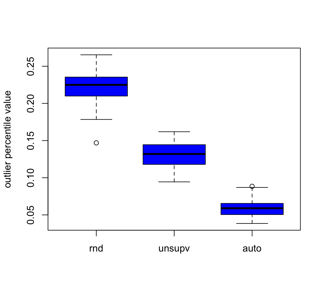

Regression problem

data(BostonHousing, package = "mlbench")

## call varpro first and then isopro
o <- varpro(medv~., BostonHousing)
o.iso <- isopro(o)

## identify data with extreme percentiles
print(BostonHousing[o.iso$howbad <= quantile(o.iso$howbad, .01),])

       crim zn indus chas   nox    rm   age    dis rad tax ptratio      b lstat medv
143 3.32105  0 19.58    1 0.871 5.403 100.0 1.3216   5 403    14.7 396.90 26.82 13.4
145 2.77974  0 19.58    0 0.871 4.903  97.8 1.3459   5 403    14.7 396.90 29.29 11.8
481 5.82401  0 18.10    0 0.532 6.242  64.7 3.4242  24 666    20.2 396.90 10.74 23.0
482 5.70818  0 18.10    0 0.532 6.750  74.9 3.3317  24 666    20.2 393.07  7.74 23.7
483 5.73116  0 18.10    0 0.532 7.061  77.0 3.4106  24 666    20.2 395.28  7.01 25.0
484 2.81838  0 18.10    0 0.532 5.762  40.3 4.0983  24 666    20.2 392.92 10.42 21.8

Supervised isopro analysis - direct call using formula/data

data(BostonHousing, package = "mlbench")

## direct approach uses formula and data options
o.iso <- isopro(formula=medv~., data=BostonHousing)

## identify data with extreme percentiles
print(BostonHousing[o.iso$howbad <= quantile(o.iso$howbad, .01),])

       crim zn indus chas   nox    rm  age    dis rad tax ptratio      b lstat medv
162 1.46336  0 19.58    0 0.605 7.489 90.8 1.9709   5 403    14.7 374.43  1.73   50
163 1.83377  0 19.58    1 0.605 7.802 98.2 2.0407   5 403    14.7 389.61  1.92   50
164 1.51902  0 19.58    1 0.605 8.375 93.9 2.1620   5 403    14.7 388.45  3.32   50
167 2.01019  0 19.58    0 0.605 7.929 96.2 2.0459   5 403    14.7 369.30  3.70   50
284 0.01501 90  1.21    1 0.401 7.923 24.8 5.8850   1 198    13.6 395.52  3.16   50
371 6.53876  0 18.10    1 0.631 7.016 97.5 1.2024  24 666    20.2 392.05  2.96   50

Unsupervised problem

## load data, make three of the classes into outliers
data(Satellite, package = "mlbench")
is.outlier <- is.element(Satellite$classes,
                         c("damp grey soil", "cotton crop", "vegetation stubble"))

## remove class labels, make unsupervised data
x <- Satellite[, names(Satellite)[names(Satellite) != "classes"]]

## isopro calls
i.rnd <- isopro(data=x, method = "rnd", sampsize=32)
i.uns <- isopro(data=x, method = "unsupv", sampsize=32)
i.aut <- isopro(data=x, method = "auto", sampsize=32)

## AUC and precision recall (computed using true class label information)
perf <- cbind(get.iso.performance(is.outlier,i.rnd$howbad),
              get.iso.performance(is.outlier,i.uns$howbad),
              get.iso.performance(is.outlier,i.aut$howbad))
colnames(perf) <- c("rnd", "unsupv", "auto")
print(perf)

             rnd    unsupv      auto
auc    0.5940483 0.8233815 0.7266512
pr.auc 0.5268934 0.7726910 0.6562785

Cite this vignette as
M. Lu, A. Shear, U. B. Kogalur, and H. Ishwaran. 2025. “isopro: identifying anomalous data vignette.” http://www.varprotools.org/articles/isopro.html.

@misc{LuIsopro,
    author = "Min Lu and Aster Shear and Udaya B. Kogalur and Hemant Ishwaran",
    title = {{isopro}: Identifying Anomalous Data vignette},
    year = {2025},
    url = {http://www.varprotools.org/articles/isopro.html},
    howpublished = "\url{http://www.varprotools.org/articles/isopro.html}",
    note = "[accessed date]"
}

1. Liu FT, Ting KM, Zhou Z-H. Isolation forest. In: 2008 eighth ieee international conference on data mining. IEEE; 2008. p. 413–22.