varPro for unsupervised problems
Min Lu (luminwin@gmail.com)
Lili Zhou (lxz516@miami.edu)
Aster Shear (aster.shear@gmail.com)
Udaya B. Kogalur (ubk@kogalur.com)
Hemant Ishwaran
(hemant.ishwaran@gmail.com)
2026-04-01
unsupervise.Rmd
Introduction
Unsupervised feature selection plays a vital role in high-dimensional data analysis, especially in fields such as bioinformatics, imaging, and text mining, where labeled outcomes are often unavailable or costly to obtain. In the absence of supervision, identifying informative variables becomes a fundamentally different and more challenging task: without a response to guide selection, variable importance must be inferred from the intrinsic structure of the data itself.
We address this challenge by extending the Variable Priority (VarPro) framework, originally developed for supervised learning, to the unsupervised domain. The resulting approach, known as Unsupervised Variable Priority (UVarPro), reframes feature selection as a sequence of localized two-class classification tasks, where the class labels arise from rule-based data partitions and their complement regions. This transformation introduces a layer of supervision grounded in statistical dependence and Bayes’ theorem, enabling principled importance estimation without labeled data.
Unlike purely heuristic approaches based on variance or clustering alignment, UVarPro draws from a more formal notion of informativeness: a variable is considered a signal if it explains the joint structure of the data and contributes to dependencies among features. This aligns with the concept of a Markov blanket in graphical models, where a minimal set of variables renders others conditionally independent. By leveraging this principle, UVarPro selects variables that preserve essential structure while filtering out noise.
UVarPro is implemented by the uvarpro function which
provides multiple strategies for unsupervised forest construction,
controlled by the method argument:
method = "auto"(default): Constructs a random forest autoencoder by regressing selected variables against themselves. This specialized multivariate forest effectively learns the internal structure of the data but may be slower on large datasets.method = "unsupv": Builds forests using standard unsupervised random forest techniques that do not rely on any response variable. This approach offers a good balance between scalability and structural fidelity.method = "rnd": Constructs forests using pure random splitting, independent of data-driven criteria. While this sacrifices structural precision, it offers the fastest performance and is useful for extremely large datasets.
Feature importance in uvarpro is quantified using an
entropy-based criterion derived from the overall variability explained
by each variable. Users may also supply custom entropy functions to
tailor the importance scoring mechanism to specific applications. See
the examples below.
For further details, see Zhou, Lu and Ishwaran (2025). Variable Priority for Unsupervised Variable Selection.
A quick start
library(varPro)
data(BostonHousing, package = "mlbench")

## default call
o <- uvarpro(BostonHousing)
print(importance(o))

             mean       std         z
nox     0.5880322 0.3838791 1.5318162
indus   0.4964445 0.3893825 1.2749533
rad     0.4051130 0.3518696 1.1513157
zn      0.4124063 0.4104604 1.0047407
medv    0.3700886 0.4275897 0.8655226
tax     0.2813970 0.3510989 0.8014749
crim    0.2791197 0.3866170 0.7219540
dis     0.2617584 0.3878109 0.6749641
lstat   0.2666589 0.3990492 0.6682358
ptratio 0.2297203 0.3440373 0.6677192
rm      0.2032958 0.3678408 0.5526733
age     0.1778247 0.3459164 0.5140685
b       0.0000000 0.0000000       NaN
chas    0.0000000 0.0000000       NaN


## unsupervised splitting
o <- uvarpro(BostonHousing, method = "unsupv")
print(importance(o))

             mean       std         z
nox     0.4869640 0.3995163 1.2188839
indus   0.4495944 0.4044867 1.1115182
lstat   0.4240813 0.4392637 0.9654369
crim    0.3803382 0.3983700 0.9547361
dis     0.3802262 0.4123258 0.9221499
tax     0.3220476 0.3811110 0.8450231
ptratio 0.3191808 0.3920556 0.8141211
medv    0.3302492 0.4193045 0.7876120
rm      0.3270985 0.4244647 0.7706141
rad     0.2503864 0.3309411 0.7565889
age     0.3014338 0.4085133 0.7378802
chas    0.2578039 0.3717827 0.6934263
zn      0.2466710 0.3703855 0.6659845
b       0.0000000 0.0000000       NaN
Example with Factors
## load the data
data(BostonHousing, package = "mlbench")

## convert some of the features to factors
Boston <- BostonHousing
Boston$zn <- factor(Boston$zn)
Boston$chas <- factor(Boston$chas)
Boston$lstat <- factor(round(0.2 * Boston$lstat))
Boston$nox <- factor(round(20 * Boston$nox))
Boston$rm <- factor(round(Boston$rm))

## call unsupervised varpro and print importance
print(importance(o <- uvarpro(Boston)))

              mean       std         z
indus   0.54117940 0.3271978 1.6539825
rm6     0.56326599 0.3975106 1.4169835
zn0     0.51511629 0.3794794 1.3574289
rad     0.36567070 0.3642130 1.0040022
tax     0.26527079 0.3446583 0.7696632
dis     0.28795676 0.3760424 0.7657561
lstat1  0.25008573 0.3660272 0.6832436
medv    0.24229301 0.3756820 0.6449418
ptratio 0.18427676 0.3168359 0.5816159
crim    0.18407113 0.3258101 0.5649645
nox8    0.17606129 0.3185826 0.5526393
nox11   0.11161593 0.2519212 0.4430588
nox9    0.08109181 0.2257001 0.3592901
nox12   0.06632392 0.1892204 0.3505114
nox10   0.07201069 0.2107668 0.3416604
nox17   0.06073111 0.1777529 0.3416604
age     0.00000000 0.0000000       NaN
chas    0.00000000 0.0000000       NaN
lstat0  0.00000000 0.0000000       NaN
lstat2  0.00000000 0.0000000       NaN
lstat3  0.00000000 0.0000000       NaN
lstat6  0.00000000 0.0000000       NaN
nox13   0.00000000 0.0000000       NaN
nox14   0.00000000 0.0000000       NaN
rm5     0.00000000 0.0000000       NaN
rm7     0.00000000 0.0000000       NaN
rm8     0.00000000 0.0000000       NaN
zn12.5  0.00000000 0.0000000       NaN
zn20    0.00000000 0.0000000       NaN
zn28    0.00000000 0.0000000       NaN
zn75    0.00000000 0.0000000       NaN

## get top variables
get.topvars(o)

 [1] "indus"   "rm6"     "zn0"     "rad"     "tax"     "dis"     "lstat1"  "medv"
 [9] "ptratio" "crim"    "nox8"    "nox11"   "nox9"    "nox12"   "nox10"   "nox17"
[17] "age"     "chas"    "lstat0"  "lstat2"  "lstat3"  "lstat6"  "nox13"   "nox14"
[25] "rm5"     "rm7"     "rm8"     "zn12.5"  "zn20"    "zn28"    "zn75"

## map importance values back to original features
print(get.orgvimp(o))

   variable         z
3     indus 1.6539825
6        rm 1.4169835
2        zn 1.3574289
9       rad 1.0040022
10      tax 0.7696632
8       dis 0.7657561
12    lstat 0.6832436
13     medv 0.6449418
11  ptratio 0.5816159
1      crim 0.5649645
5       nox 0.5526393
4      chas 0.0000000
7       age 0.0000000

## same as above ... but for all variables
print(get.orgvimp(o, pretty = FALSE))

     crim        zn     indus      chas       nox        rm       age       dis       rad
0.5649645 1.3574289 1.6539825 0.0000000 0.5526393 1.4169835 0.0000000 0.7657561 1.0040022
      tax   ptratio         b     lstat      medv
0.7696632 0.5816159 0.0000000 0.6832436 0.6449418
Custom Importance Functions – Option 1: Inline Entropy
VarPro allows users to define a custom importance function through
the (hidden) entropy argument. This function is evaluated
internally during forest construction.
The custom function must return a list with two elements: 1. A scalar
importance value. 2. An entropy list containing the
comp and oob membership vectors.
Example:
my.entropy <- function(xC, xO, ...) {
  wss <- mean(apply(rbind(xO, xC), 2, sd, na.rm = TRUE))
  bss <- mean(apply(xO, 2, sd, na.rm = TRUE)) +
         mean(apply(xC, 2, sd, na.rm = TRUE))
  imp <- 0.5 * bss / wss

  entropy <- list(comp = list(...)$compMembership,
                  oob  = list(...)$oobMembership)

  list(imp = imp, entropy)
}

o <- uvarpro(BostonHousing, entropy = my.entropy)
print(importance(o))

             mean       std         z
nox     0.5689125 0.3900506 1.4585608
indus   0.5087139 0.3900071 1.3043709
rad     0.3504640 0.3520091 0.9956106
zn      0.3997953 0.4147441 0.9639565
medv    0.4126304 0.4310544 0.9572582
tax     0.3490256 0.3727909 0.9362502
crim    0.3446691 0.3990397 0.8637464
dis     0.2564835 0.3807887 0.6735587
ptratio 0.2151499 0.3324902 0.6470863
lstat   0.2429619 0.3907914 0.6217177
age     0.2182291 0.3743837 0.5829022
rm      0.1556733 0.3331967 0.4672112
b       0.0000000 0.0000000       NaN
chas    0.0000000 0.0000000       NaN
Custom Importance Functions – Option 2: Post-hoc Construction
As an alternative, users can compute variable importance
after model fitting by working directly with the
$entropy output. This approach gives full control over the
definition of importance scores.
data(BostonHousing, package = "mlbench")
o <- uvarpro(BostonHousing[-(1:5), ])
beta <- get.beta.entropy(o)
print(beta[1:5, 1:5])

              crim         zn     indus         nox        rm
crim  0.0000000000 0.10040957 1.0045794  3.79113503 0.2526244
zn    0.2941171442 0.00000000 1.2070505 11.04463518 0.8142999
indus 0.3386272960 1.13606934 0.0000000  7.88050758 1.3338613
nox   0.9156186492 0.64743152 1.5504832  0.00000000 0.9111166
rm    0.0001214442 0.05192334 0.1060687  0.02870288 0.0000000

sdependent(beta)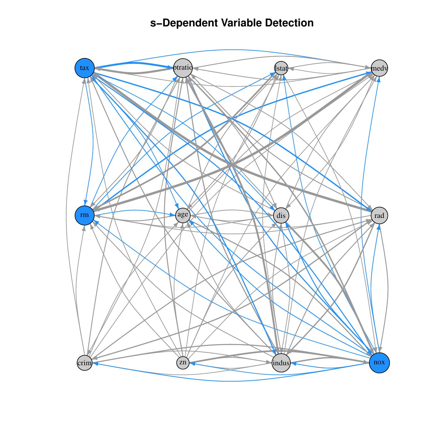
In the above example of function get.beta.entropy, the
th
row serves as a ensembled regression model, representing the importance
scores for the
th
variable. The function sdependent provides S-dependence map
of the L1-logistic coefficient matrix — reveals variable dependence
structure without labels.
For large datasets, consider using parallel::mclapply to
improve computation time.
| Summary |
| Both approaches offer flexibility in defining importance scores tailored to domain-specific objectives. Option 1 is more integrated, while Option 2 offers full post-processing control. |
Cite this vignette as
M. Lu, L. Zhou, A.
Shear, U. B. Kogalur, and H. Ishwaran. 2024. “varPro: variable selection
for unsupervised problems vignette.” http://www.varprotools.org/articles/unsupervise.html.
@misc{HemantUvarpro,
    author = "Min Lu and Lili Zhou and Aster Shear and Udaya B. Kogalur and Hemant Ishwaran",
    title = {{varPro}: variable selection for unsupervised problems vignette},
    year = {2024},
    url = {http://www.varprotools.org/articles/unsupervise.html},
    howpublished = "\url{http://www.varprotools.org/articles/unsupervise.html}",
    note = "[accessed date]"
}